Controlling the standard deviation of activity

This example illustrates how the standard deviation (SD) of source activity can be manipulated.

# sphinx_gallery_thumbnail_path = '_static/example_stubs/thumb/sphx_glr_04_plot_brain_std_thumb.png'

import matplotlib.pyplot as plt
import mne
import numpy as np

from mne.datasets import sample

from meegsim.location import select_random
from meegsim.simulate import SourceSimulator
from meegsim.waveform import narrowband_oscillation

First, we load the head model and associated source space:

# Paths
subjects_dir = sample.data_path() / "subjects"
data_path = sample.data_path() / "MEG" / "sample"
fwd_path = data_path / "sample_audvis-meg-eeg-oct-6-fwd.fif"
raw_path = data_path / "sample_audvis_raw.fif"

# Load the prerequisites: fwd, src, and info
fwd = mne.read_forward_solution(fwd_path)
fwd = mne.convert_forward_solution(fwd, force_fixed=True)
raw = mne.io.read_raw(raw_path)
src = fwd["src"]
info = raw.info

# Pick EEG channels only
eeg_idx = mne.pick_types(info, eeg=True)
info_eeg = mne.pick_info(info, eeg_idx)
fwd_eeg = fwd.pick_channels(info_eeg.ch_names)

Simulation parameters are listed below:

sfreq = 250
duration = 60
seed = 1234
target_snr = 4
fmin = 8
fmax = 12

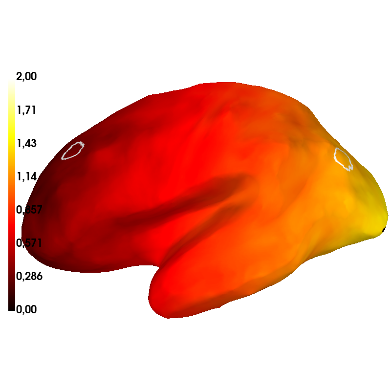
To illustrate the effect, we set the SD based on the y-position of the sources, with higher SDs for parieto-occipital areas. By wrapping the SD values in a mne.SourceEstimate object, we can set the SD for whole sources at once even if there actual positions are generated randomly. In this case, however, we pick the source locations manually to show the effect better with one frontal and one occipital source:

ypos = np.hstack([s["rr"][s["inuse"] > 0, 1] for s in src])
std = 1 - 8 * ypos
vertno = [s["vertno"] for s in src]
std_stc = mne.SourceEstimate(
    data=std, vertices=vertno, tmin=0, tstep=0.01, subject="sample"
)
source_vertno = [126371, 10957]  # frontal & occipital

# The resulting spatial distribution of SD along with chosen locations for patch
# sources (white borders) are shown below:

patches = mne.grow_labels(
    subject="sample",
    seeds=source_vertno,
    extents=10,
    hemis=[0, 0],
    subjects_dir=subjects_dir,
)
brain = std_stc.plot(
    subject="sample",
    subjects_dir=subjects_dir,
    hemi="lh",
    views="lat",
    clim=dict(kind="value", lims=[0, 1, 2]),
    transparent=False,
    background="white",
)
for patch in patches:
    brain.add_label(patch, color="white", borders=True)

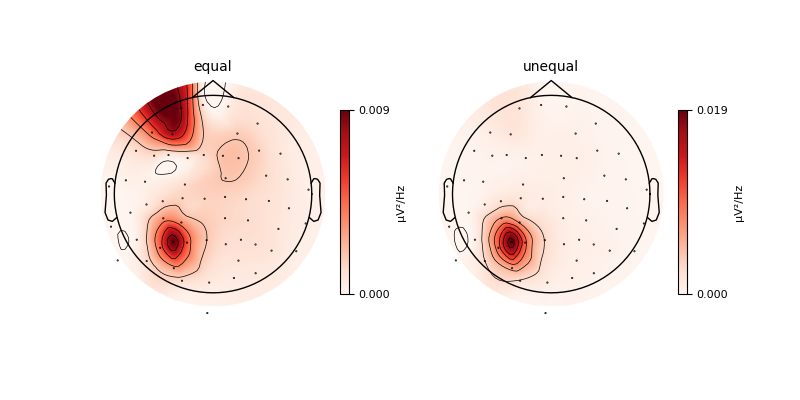
Below, we create two identical simulations except for the standard deviation (std argument of add_patch_sources() call). We then illustrate the difference in the topomap of alpha power betweeen two cases: equal SD for all sources (std=1.0) vs. custom variance based on std_stc. As expected, occipital source dominates the topomap when the custom SD is used:

fig, axes = plt.subplots(ncols=2, figsize=(8, 4))
for ax, std, case in zip(axes, [1.0, std_stc], ["equal", "unequal"]):
    sim = SourceSimulator(src)

    sim.add_noise_sources(location=select_random, location_params=dict(n=10))

    # Use manually selected vertices, put all sources in the left hemisphere
    sim.add_patch_sources(
        location=[(0, v) for v in source_vertno],
        waveform=narrowband_oscillation,
        location_params=dict(n=3),
        waveform_params=dict(fmin=fmin, fmax=fmax),
        std=std,
        extents=10,
        subject="sample",
        subjects_dir=subjects_dir,
    )

    sc = sim.simulate(
        sfreq,
        duration,
        fwd=fwd,
        snr_global=target_snr,
        snr_params=dict(fmin=fmin, fmax=fmax),
        random_state=seed,
    )
    raw = sc.to_raw(fwd, info, sensor_noise_level=0.05)

    spec = raw.compute_psd(n_fft=sfreq, n_overlap=sfreq // 2, n_per_seg=sfreq)
    spec.plot_topomap(bands={case: (8, 12)}, axes=ax)