Adjustment of global SNR

This example shows how the global SNR can be adjusted.

import mne
import matplotlib.pyplot as plt

from mne.datasets import sample

from meegsim.location import select_random
from meegsim.simulate import SourceSimulator
from meegsim.waveform import narrowband_oscillation

First, we load the head model and associated source space:

# Paths
data_path = sample.data_path() / "MEG" / "sample"
fwd_path = data_path / "sample_audvis-meg-eeg-oct-6-fwd.fif"
raw_path = data_path / "sample_audvis_raw.fif"

# Load the prerequisites: fwd, src, and info
fwd = mne.read_forward_solution(fwd_path)
fwd = mne.convert_forward_solution(fwd, force_fixed=True)
raw = mne.io.read_raw(raw_path)
src = fwd["src"]
info = raw.info

# Pick EEG channels only
eeg_idx = mne.pick_types(info, eeg=True)
info_eeg = mne.pick_info(info, eeg_idx)
fwd_eeg = fwd.pick_channels(info_eeg.ch_names)

Reading forward solution from /home/docs/mne_data/MNE-sample-data/MEG/sample/sample_audvis-meg-eeg-oct-6-fwd.fif...
    Reading a source space...
    Computing patch statistics...
    Patch information added...
    Distance information added...
    [done]
    Reading a source space...
    Computing patch statistics...
    Patch information added...
    Distance information added...
    [done]
    2 source spaces read
    Desired named matrix (kind = 3523 (FIFF_MNE_FORWARD_SOLUTION_GRAD)) not available
    Read MEG forward solution (7498 sources, 306 channels, free orientations)
    Desired named matrix (kind = 3523 (FIFF_MNE_FORWARD_SOLUTION_GRAD)) not available
    Read EEG forward solution (7498 sources, 60 channels, free orientations)
    Forward solutions combined: MEG, EEG
    Source spaces transformed to the forward solution coordinate frame
    Average patch normals will be employed in the rotation to the local surface coordinates....
    Converting to surface-based source orientations...
    [done]
Opening raw data file /home/docs/mne_data/MNE-sample-data/MEG/sample/sample_audvis_raw.fif...
    Read a total of 3 projection items:
        PCA-v1 (1 x 102)  idle
        PCA-v2 (1 x 102)  idle
        PCA-v3 (1 x 102)  idle
    Range : 25800 ... 192599 =     42.956 ...   320.670 secs
Ready.

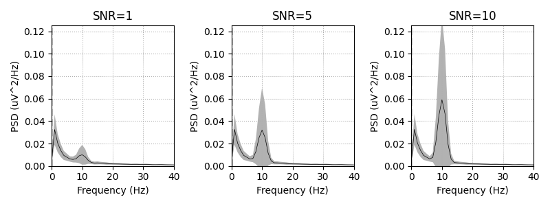
We simulate the same configuration (100 noise sources and 3 point sources) several times with different levels of SNR. As shown in the picture below, the average alpha power increases relative to the 1/f level with higher SNR:

# Simulation parameters
sfreq = 250
duration = 60
seed = 123

fig, axes = plt.subplots(ncols=3, figsize=(8, 3))
snr_values = [1, 5, 10]

for i_snr, target_snr in enumerate(snr_values):
    sim = SourceSimulator(src)

    # Select some vertices randomly
    sim.add_point_sources(
        location=select_random,
        waveform=narrowband_oscillation,
        location_params=dict(n=3),
        waveform_params=dict(fmin=8, fmax=12),
        names=["s1", "s2", "s3"],
    )

    sim.add_noise_sources(location=select_random, location_params=dict(n=100))

    sc = sim.simulate(
        sfreq,
        duration,
        fwd=fwd,
        snr_global=target_snr,
        snr_params=dict(fmin=8, fmax=12),
        random_state=seed,
    )
    raw = sc.to_raw(fwd, info)

    spec = raw.compute_psd(fmax=40, n_fft=sfreq, n_overlap=sfreq // 2, n_per_seg=sfreq)
    spec.plot(average=True, dB=False, axes=axes[i_snr], amplitude=False)

    axes[i_snr].set_title(f"SNR={target_snr}")
    axes[i_snr].set_xlabel("Frequency (Hz)")
    axes[i_snr].set_ylabel("PSD (uV^2/Hz)")
    axes[i_snr].set_ylim([0, 0.125])

fig.tight_layout()

Projecting source estimate to sensor space...
[done]
Creating RawArray with float64 data, n_channels=59, n_times=15000
    Range : 0 ... 14999 =      0.000 ...    59.996 secs
Ready.
Effective window size : 1.000 (s)
Plotting power spectral density (dB=False).
Projecting source estimate to sensor space...
[done]
Creating RawArray with float64 data, n_channels=59, n_times=15000
    Range : 0 ... 14999 =      0.000 ...    59.996 secs
Ready.
Effective window size : 1.000 (s)
Plotting power spectral density (dB=False).
Projecting source estimate to sensor space...
[done]
Creating RawArray with float64 data, n_channels=59, n_times=15000
    Range : 0 ... 14999 =      0.000 ...    59.996 secs
Ready.
Effective window size : 1.000 (s)
Plotting power spectral density (dB=False).