Plotting the configuration

This example illustrates how to plot the simulated source configuration.

# sphinx_gallery_thumbnail_path = '_static/example_stubs/thumb/sphx_glr_02_plot_brain_configuration_thumb.png'

import mne

from mne.datasets import sample

from meegsim.location import select_random
from meegsim.simulate import SourceSimulator
from meegsim.waveform import narrowband_oscillation

First, we load all the prerequisites for our simulation and restrict to the EEG channels only

# Paths
subjects_dir = sample.data_path() / "subjects"
data_path = sample.data_path() / "MEG" / "sample"
fwd_path = data_path / "sample_audvis-meg-eeg-oct-6-fwd.fif"
raw_path = data_path / "sample_audvis_raw.fif"

print(subjects_dir)

# Load the prerequisites: fwd, src, and info
fwd = mne.read_forward_solution(fwd_path)
raw = mne.io.read_raw(raw_path)
src = fwd["src"]
info = raw.info

# Pick EEG channels only
eeg_idx = mne.pick_types(info, eeg=True)
info_eeg = mne.pick_info(info, eeg_idx)
fwd_eeg = fwd.pick_channels(info_eeg.ch_names)

Below we define the simulation itself. In this case, we place 50 noise (1/f) sources and add a couple of point and patch sources for demonstration purposes. All sources are placed randomly.

# Simulation parameters
sfreq = 100  # in Hz
duration = 60  # in seconds

# Initialize
sim = SourceSimulator(src)

# Add 50 noise sources with random locations
sim.add_noise_sources(location=select_random, location_params=dict(n=50))

# Add point sources
sim.add_point_sources(
    location=select_random,
    location_params=dict(n=3),
    waveform=narrowband_oscillation,
    waveform_params=dict(fmin=8, fmax=12),
)

# Add patch sources
sim.add_patch_sources(
    location=select_random,
    location_params=dict(n=3),
    waveform=narrowband_oscillation,
    waveform_params=dict(fmin=8, fmax=12),
    extents=[10, 20, 50],
    subject="sample",
    subjects_dir=subjects_dir,
)

Now we simulate the configuration with an arbitrary level of global SNR:

sc = sim.simulate(
    sfreq,
    duration,
    fwd=fwd_eeg,
    snr_global=3,
    snr_params=dict(fmin=8, fmax=12),
    random_state=1234,
)

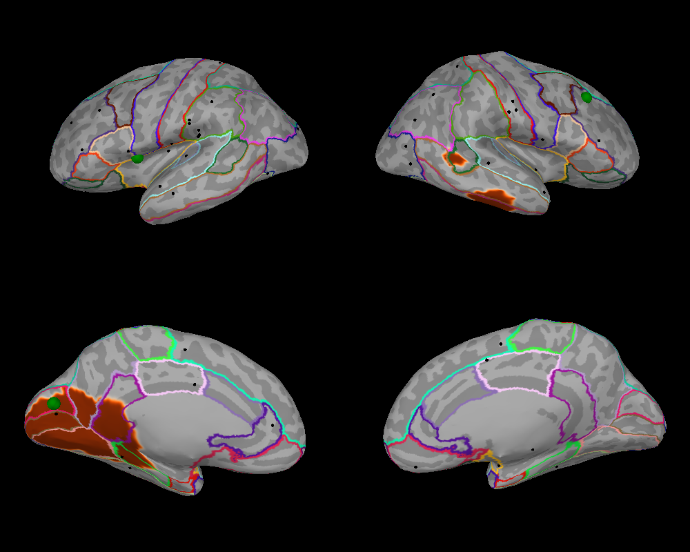
We can now plot the source configuration using the dedicated method plot() of the SourceConfiguration class. The method returns a Brain object, which can be used to plot additional information, e.g., parcellation of interest.

brain = sc.plot(
    scale_factors=dict(point=1.25),
    subject="sample",
    subjects_dir=subjects_dir,
    size=(1000, 800),
    background="black",
    hemi="split",
    views=["lat", "med"],
)
brain.add_annotation("aparc")