Random state and reproducibility

This example showcases how reproducible source configurations can be achieved by fixing the random state when simulating.

import matplotlib.pyplot as plt
import mne
import numpy as np

from mne.datasets import sample

from meegsim.coupling import ppc_shifted_copy_with_noise
from meegsim.location import select_random
from meegsim.waveform import narrowband_oscillation
from meegsim.simulate import SourceSimulator

First, we load the head model and associated source space:

# Paths
data_path = sample.data_path() / "MEG" / "sample"
fwd_path = data_path / "sample_audvis-meg-eeg-oct-6-fwd.fif"
raw_path = data_path / "sample_audvis_raw.fif"

# Load the prerequisites: fwd, src, and info
fwd = mne.read_forward_solution(fwd_path)
fwd = mne.convert_forward_solution(fwd, force_fixed=True)
raw = mne.io.read_raw(raw_path)
src = fwd["src"]
info = raw.info

# Pick EEG channels only
eeg_idx = mne.pick_types(info, eeg=True)
info_eeg = mne.pick_info(info, eeg_idx)
fwd_eeg = fwd.pick_channels(info_eeg.ch_names)

Reading forward solution from /home/docs/mne_data/MNE-sample-data/MEG/sample/sample_audvis-meg-eeg-oct-6-fwd.fif...
    Reading a source space...
    Computing patch statistics...
    Patch information added...
    Distance information added...
    [done]
    Reading a source space...
    Computing patch statistics...
    Patch information added...
    Distance information added...
    [done]
    2 source spaces read
    Desired named matrix (kind = 3523 (FIFF_MNE_FORWARD_SOLUTION_GRAD)) not available
    Read MEG forward solution (7498 sources, 306 channels, free orientations)
    Desired named matrix (kind = 3523 (FIFF_MNE_FORWARD_SOLUTION_GRAD)) not available
    Read EEG forward solution (7498 sources, 60 channels, free orientations)
    Forward solutions combined: MEG, EEG
    Source spaces transformed to the forward solution coordinate frame
    Average patch normals will be employed in the rotation to the local surface coordinates....
    Converting to surface-based source orientations...
    [done]
Opening raw data file /home/docs/mne_data/MNE-sample-data/MEG/sample/sample_audvis_raw.fif...
    Read a total of 3 projection items:
        PCA-v1 (1 x 102)  idle
        PCA-v2 (1 x 102)  idle
        PCA-v3 (1 x 102)  idle
    Range : 25800 ... 192599 =     42.956 ...   320.670 secs
Ready.

For this example, we place some sources in random locations and set up one connectivity edge. Unless the random_state is fixed, all randomly generated components (location, waveform, coupling) will differ between simulated configurations. With a fixed random_state, the results become reproducible.

sim = SourceSimulator(src)

# Select some vertices randomly
n_sources = 3
sim.add_point_sources(
    location=select_random,
    waveform=narrowband_oscillation,
    location_params=dict(n=n_sources),
    waveform_params=dict(fmin=8, fmax=12),
    names=[str(i) for i in range(n_sources)],
)
sim.set_coupling(
    ("0", "1"),
    method=ppc_shifted_copy_with_noise,
    phase_lag=np.pi / 2,
    coh=0.5,
    fmin=8,
    fmax=12,
    band_limited=False,
)

We simulate three configurations, the first and the last one of them have the same random_state:

sfreq = 250
duration = 60
sc1 = sim.simulate(sfreq=sfreq, duration=duration, random_state=123)
sc2 = sim.simulate(sfreq=sfreq, duration=duration, random_state=456)
sc3 = sim.simulate(sfreq=sfreq, duration=duration, random_state=123)

First, we can check the locations (vertno) of the simulated sources:

for i, sc in enumerate([sc1, sc2, sc3]):
    print(f"Configuration {i+1}: {[int(s.vertno) for s in sc._sources.values()]}")

Configuration 1: [126025, 14801, 45559]
Configuration 2: [36679, 69544, 10915]
Configuration 3: [126025, 14801, 45559]

For the source with name "1", we additionally plot the waveform in all three configurations:

n_samples_to_plot = 1000
fig, axes = plt.subplots(nrows=3, figsize=(8, 6), layout="constrained")
for i, (ax, sc) in enumerate(zip(axes, [sc1, sc2, sc3])):
    waveform = np.squeeze(sc["1"].waveform)
    ax.plot(sc.times[:n_samples_to_plot], waveform[:n_samples_to_plot])
    ax.set_xlabel("Time (s)")
    ax.set_ylabel("Amplitude (nAm)")
    ax.set_title(f"Configuration {i+1} | random_state={sc.random_state}")

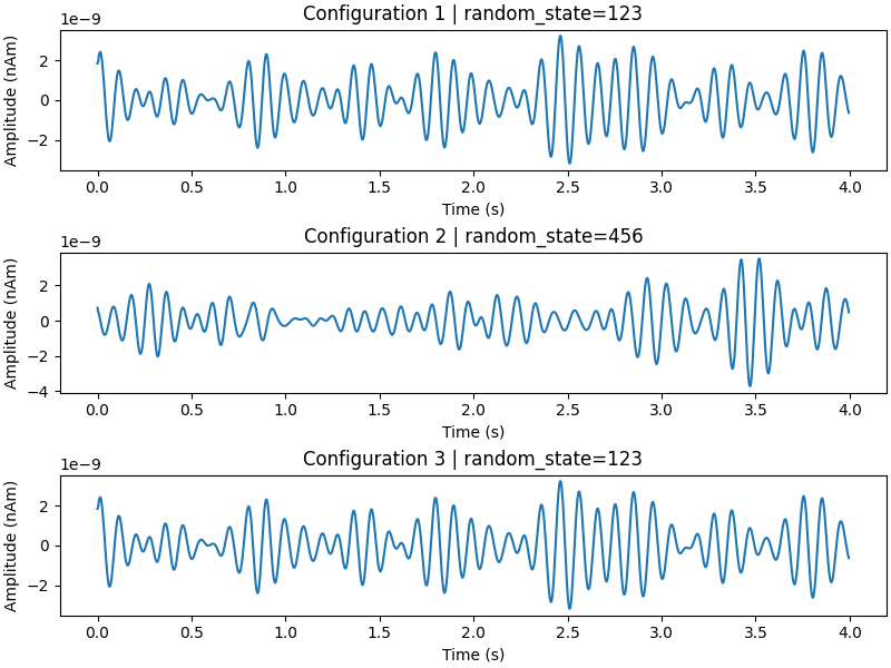
As expected, both locations and waveforms of the simulated sources are the same for configurations 1 and 3 but different for configuration 2.