Phase-phase coupling based on von Mises distribution

This example illustrates how the choice of kappa affects the obtained phase-phase coupling if the ppc_von_mises() method based on the von Mises distribution is used.

import numpy as np
from harmoni.extratools import compute_plv
from matplotlib import pyplot as plt

from meegsim.coupling import ppc_von_mises
from meegsim.waveform import narrowband_oscillation

To illustrate the effect, we consider a range of values from 0.01 to 10 for kappa, performing several simulations for each value. In addition, we vary the length of the simulated data:

lengths = [10, 30, 60]
n_kappas = 11
n_runs = 25
kappas = np.logspace(-2, 1, n_kappas)
sfreq = 250
fmin = 8
fmax = 12

For each considered setting (kappa, data length), we randomly generate a narrowband alpha (8-12 Hz) oscillation and a coupled oscillation with the mean phase lag of \({\pi}/2\). We then estimate the phase-locking value (PLV) of the simulated oscillations and plot the mean PLV (black line) as well as its standard deviation (shaded region: +-1.96SD):

fig, axes = plt.subplots(ncols=len(lengths), figsize=(9, 4), layout="constrained")
for ax, length in zip(axes, lengths):
    times = np.arange(0, length, 1 / sfreq)
    waveform = narrowband_oscillation(1, times, fmin=fmin, fmax=fmax)

    phase_lag = np.pi / 4
    plv = np.zeros((n_runs, n_kappas))
    for i_run in range(n_runs):
        for i_kappa, kappa in enumerate(kappas):
            result = ppc_von_mises(
                waveform, sfreq, phase_lag, kappa=kappa, fmin=fmin, fmax=fmax
            )
            cplv = compute_plv(waveform, result, m=1, n=1, plv_type="complex")
            plv[i_run, i_kappa] = np.abs(cplv)[0][0]

    plv_mean = np.mean(plv, axis=0)
    plv_sd = np.std(plv, axis=0)
    ax.plot(kappas, plv_mean, c="k", linewidth=1.5)
    ax.fill_between(
        kappas, plv_mean - 1.96 * plv_sd, plv_mean + 1.96 * plv_sd, color="grey"
    )
    ax.set_xscale("log")
    ax.set_xticks([0.01, 0.1, 1, 10])
    ax.set_xticklabels([0.01, 0.1, 1, 10])
    ax.set_ylim([0, 1])
    ax.set_xlabel("Kappa")
    ax.set_ylabel("PLV")
    ax.set_title(f"duration = {length} s")

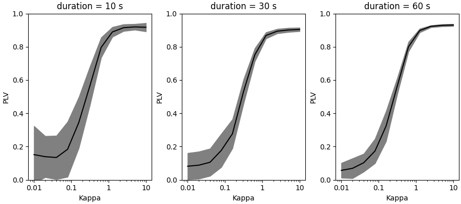
As shown in the plots above, kappa is monotoneously related to the resulting PLV between coupled time series. This allows for flexible control of coupling, and these plots can be used as reference when picking a suitable value of kappa. For lower values of kappa and shorter recordings, the estimated connectivity has a non-zero noise floor (mean does not reach 0) and becomes less stable (the SD becomes larger).

If the connectivity measure depends on both amplitude and phase (e.g., coherence), its estimated value will also depend on the correspondence between amplitude envelopes of the time series.